Statistical Process Control for .NET Developers

Most teams already collect operational metrics. The hard part is spotting when a process is changing before it turns into an outage, regression, or support ticket. A moving average can hide drift. A dashboard can show that numbers are “still in range” while the process is quietly getting worse.

That is where statistical process control can help.

The insight: thresholds vs. control limits

Most systems today rely on fixed thresholds such as SLAs or alert limits.

Thresholds tell you when you have already broken a promise.

Control limits answer a different question. They tell you whether your process is still behaving like itself.

A system can be within specification and still be drifting, shifting, or becoming unstable. That is exactly the gap SPC is designed to close. It focuses on detecting non-random behavior, not just threshold breaches.

The Numerics.NET SPC API is designed for this kind of workflow. It is calculation-first. You fit a baseline from historical data, then apply that frozen baseline to new observations. You can render the results however you like. In this example, we will use ScottPlot 5 from a simple console app to generate a PNG.

We will work with a synthetic server latency dataset in two phases:

• Phase I: use stable historical data to learn what “normal” looks like
• Phase II: apply that frozen baseline to new samples and look for signals

That is a much more realistic operational workflow than mixing stable and unstable data in one retrospective batch.

The scenario

Imagine you are tracking request latency for a backend service. For a while, the service is stable. Then a rollout changes something subtle. Requests are still within the SLA, and none of the new values look dramatic on their own, but they are all slightly higher than the old baseline.

That is exactly the kind of shift SPC is good at surfacing.

For this example:

• the first twenty observations form a stable baseline
• the next eight observations are all a little higher

That lets us show the real value of SPC: the process can still be “acceptable” in a business sense while already signaling that it is no longer behaving like the old process.

Add the packages

You only need two packages:

dotnet add package Numerics.NET
dotnet add package ScottPlot

The complete example

Here is a complete Program.cs that:

• fits an I-MR baseline from Phase I data
• deploys and serializes that baseline
• restores it later
• applies it to Phase II data
• evaluates Western Electric rules on the monitored data
• renders a chart to latency-i-chart.png

using System;
using System.Collections.Generic;
using System.Linq;

using Numerics.NET;
using Numerics.NET.Statistics.ProcessControl;

using ScottPlot;

License.Verify("49610-02352-19605-38737");

Vector<double> baselineMs =
    [
        120.1, 119.8, 120.4, 120.0, 119.7, 120.3, 119.9, 120.2,
        120.1, 119.6, 120.5, 119.8, 120.0, 120.3, 119.9, 120.4,
        120.2, 119.7, 120.1, 119.8
    ];

// Phase I: fit a baseline from historical stable data.
var baseline = new IndividualsMovingRangeChartSet(baselineMs);
baseline.Analyze();

var baselineSeries = baseline.IndividualsSeries;

Console.WriteLine(
    $"Baseline I chart: CL={baselineSeries.CenterLine:F2} " +
    $"UCL={baselineSeries.UpperControlLimit:F2} " +
    $"LCL={baselineSeries.LowerControlLimit:F2}");

// Persist the deployed baseline for later use.
string json = baseline.Deploy().ToJson();

// Phase II: restore the baseline and apply it to new observations.
var deployed = IndividualsMovingRangeChartSet.FromJson(json);

Vector<double> newLatencyMs =
    [
        120.0, 120.1, 119.9, 120.2, 120.4, 120.7, 121.0, 121.4
    ];

var monitored = deployed.Apply(newLatencyMs);
var monitoredSeries = monitored.IndividualsSeries;

// Use a rule set that gives a clean signal here: 8 points on one side.
var evaluation = monitoredSeries.EvaluateRules(ControlRuleSets.WesternElectric);

bool stable = !evaluation.HasViolations;
Console.WriteLine($"Phase II stable: {stable}");

if (evaluation.HasViolations)
{
    RuleViolation first = evaluation.Violations[0];
    Console.WriteLine(
    $"Signal: {first.RuleId} at sample " +
    $"{baselineMs.Length + first.TriggerIndex + 1}");
}

// x-axis values for Phase I and Phase II.
Vector<double> phase1Xs = Vector.Range(1.0, baselineMs.Length);
Vector<double> phase2Xs = Vector.Range(
    baselineMs.Length + 1.0,
    baselineMs.Length + newLatencyMs.Length);

// Render the Individuals chart using the frozen Phase I limits.
Plot plot = new();

var phase1Plot = plot.Add.Scatter(phase1Xs.ToArray(), baselineMs.ToArray());
phase1Plot.LegendText = "Phase I baseline";
phase1Plot.MarkerSize = 7;

var phase2Plot = plot.Add.Scatter(phase2Xs.ToArray(), newLatencyMs.ToArray());
phase2Plot.LegendText = "Phase II monitoring";
phase2Plot.MarkerSize = 7;

var centerLine = plot.Add.HorizontalLine(baselineSeries.CenterLine);
centerLine.Text = "Center line";
centerLine.Color = Colors.Blue;

var upperLimit = plot.Add.HorizontalLine(baselineSeries.UpperControlLimit);
upperLimit.Text = "UCL";
upperLimit.Color = Colors.Red;

var lowerLimit = plot.Add.HorizontalLine(baselineSeries.LowerControlLimit);
lowerLimit.Text = "LCL";
lowerLimit.Color = Colors.Red;

var handoff = plot.Add.VerticalLine(baselineMs.Length + 0.5);
handoff.Text = "Phase II begins";

if (evaluation.HasViolations)
{
    var flagged = plot.Add.ScatterPoints(
        phase2Xs[evaluation.TriggerIndexes].ToArray(),
        monitoredSeries.Values[evaluation.TriggerIndexes].ToArray());
    flagged.LegendText = "Signals";
    flagged.Color = Colors.Red;
    flagged.MarkerSize = 10;
}

plot.Title("Server Latency: Phase I Baseline, Phase II Monitoring");
plot.XLabel("Sample");
plot.YLabel("Latency (ms)");
plot.ShowLegend();

plot.SavePng("latency-i-chart.png", 900, 500);

Console.WriteLine("Saved chart to latency-i-chart.png");
Console.WriteLine("The moving-range series is available as monitored.MovingRangesSeries.");

Running the sample produces output like this:

Baseline I chart: CL=120.04 UCL=121.15 LCL=118.93
Phase II stable: False
Signal: PointBeyondControlLimits at sample 28
Saved chart to latency-i-chart.png
The moving-range series is available as monitored.MovingRangesSeries.

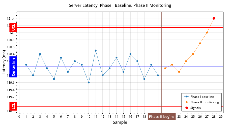
Here’s the chart that is produced:

What the code is doing

The key calls are these:

var baseline = new IndividualsMovingRangeChartSet(baselineMs);
baseline.Analyze();

string json = baseline.Deploy().ToJson();

var deployed = IndividualsMovingRangeChartSet.FromJson(json);
var monitored = deployed.Apply(newLatencyMs);

var evaluation = monitored.IndividualsSeries.EvaluateRules(ControlRuleSets.WesternElectric);

That sequence tells the story:

• build a baseline from known historical data
• deploy and persist that baseline
• restore it later
• apply it to fresh observations
• evaluate rules on the monitored series

That is the SPC lifecycle in a form that maps nicely to real applications.

Phase I vs. Phase II, without the jargon overload

SPC literature usually splits the work into two phases:

Phase I: learn the baseline

Use historical data to estimate the center line and control limits.

Phase II: monitor against the baseline

Take new data and ask: does it still look like the same process?

That is exactly what the code above does.

The first twenty latency samples teach the chart what “normal” looks like. The next eight are checked against that frozen baseline.

This matters because it avoids a common mistake: if you mix the stable and shifted data together when fitting the chart, you can blur the very change you are trying to detect.

From data points to signals

The chart shows:

• the Phase I baseline
• the Phase II monitoring points
• the frozen center line
• the frozen upper and lower control limits
• the points where a rule actually fires

In this example, the new values are only slightly higher. None of them scream “incident” on their own. But all eight Phase II points land on the same side of the old center line, which is enough to trigger the Western Electric run rule.

That is the whole point.

We are not saying “this number is large.” We are saying “this process is no longer behaving like the one we learned in Phase I.”

That is a far more useful signal in production systems.

The trigger points come directly from evaluation.TriggerIndexes, which makes it easy to highlight the actual signal locations in a chart without reconstructing them manually.

Where capability fits

Capability analysis still matters, but it is a separate question.

Control charts ask:

Is the process stable?

Capability asks:

Given a stable process, how well does it fit the specification?

That means capability is best treated as a follow-up step, not the main hook for this example.

Once you have a stable baseline, you can layer in specification limits, capability indices, and assumption diagnostics as a separate analysis path. That is especially useful when you want to move from “something changed” to “how much performance margin do we really have?”

Why this pattern works well in real .NET applications

This example uses a console app and writes a PNG, but the shape scales well:

• ingest baseline measurements from a database or telemetry store
• fit a chart with Analyze()
• deploy that baseline
• apply new data in batches as it arrives
• evaluate rules on the monitored series
• render or persist the results wherever you want

That is the value of a calculation-first API. The statistical logic stays in your application, and the visualization layer stays swappable.

Final thoughts

If you have ever wanted SPC in a .NET application without dragging in a spreadsheet workflow or a heavyweight GUI tool, this is a clean starting point.

This example uses an Individuals and Moving Range chart, but the same design extends to subgrouped variables charts such as XBar-R and XBar-S, as well as attribute charts such as p and u.

The real payoff is not just that you can draw a control chart. It is that you can model the real lifecycle of process monitoring in code:

• fit a baseline
• freeze it
• apply it to new data
• detect meaningful change early

That is a much better fit for software systems than waiting for a threshold to break and hoping the dashboard told the full story.