Kernel Density Estimation
Kernel density estimation (KDE) is a method for estimating the probability density function of a variable. The estimated distribution is taken to be the sum of appropriately scaled and positioned kernels. The bandwidth specifies how far out each observation affects the density estimate.
Kernel density estimation is implemented by the KernelDensity class in the Numerics.NET.Statistics namespace. For reusable fits, import Numerics.NET.Statistics.KernelDensityEstimation, which contains the estimate, grid, fitting options, FFT options and transformation types. KernelDensityDistribution remains with the other continuous distributions.
In the code examples, we will repeatedly use a sample generated from a mixture of two Gaussian distributions:
var norm1 = new NormalDistribution(-1, 1);
var norm2 = new NormalDistribution(1, 0.3);
var X = Vector.Join(norm1.Sample(400), norm2.Sample(100));Evaluate a Basic Density
Use EstimateGaussian(Vector<Double>, Double, Nullable<Double>) to evaluate a Gaussian density at one coordinate, or EstimateGaussian(Vector<Double>, Vector<Double>, Nullable<Double>) to evaluate a supplied vector of coordinates. Omit the bandwidth, or pass null, to select the Gaussian normal-reference width. To inspect or reuse that width, call EstimateGaussianBandwidth(Vector<Double>). An explicit bandwidth is in observation units and must be finite and positive.
EstimateEpanechnikov(Vector<Double>, Vector<Double>, Double), EstimateTriangular(Vector<Double>, Double, Double) and EstimateUniform(Vector<Double>, Double, Double) provide three compact-support alternatives. Each has scalar and vector-query overloads and requires an explicit bandwidth. Their standardized support is [-1, 1].
Vector<double> basicObservations = Vector.Create(new double[] { -1.2, -.3, 0, .4, 1.7, 2 });
Vector<double> basicQueries = Vector.Create(new double[] { -1, 0, 1 });
double basicBandwidth = KernelDensity.EstimateGaussianBandwidth(basicObservations);
double gaussianAtZero = KernelDensity.EstimateGaussian(basicObservations, 0);
Vector<double> gaussianDensities = KernelDensity.EstimateGaussian(
    basicObservations, basicQueries, bandwidth: .5);
Vector<double> epanechnikovDensities = KernelDensity.EstimateEpanechnikov(
    basicObservations, basicQueries, basicBandwidth);
double triangularAtZero = KernelDensity.EstimateTriangular(basicObservations, 0, basicBandwidth);
double uniformAtZero = KernelDensity.EstimateUniform(basicObservations, 0, basicBandwidth);These methods give every observation equal weight. Observations must be nonempty and finite. Automatic Gaussian bandwidth selection requires at least two observations with positive spread; a single observation or constant data requires an explicit bandwidth. Query vectors may be empty or unsorted. Results preserve query order and labels, and do not modify either input vector. A NaN query produces NaN; either infinity produces zero. The methods evaluate densities directly at the supplied coordinates without normalizing over those coordinates.
For a normalized custom kernel, use Estimate(Vector<Double>, Vector<Double>, Double, Func<Double, Double>) or its scalar-query overload. The delegate must be nonnegative and integrate to one over the real line. Return zero outside its support, including at infinite standardized arguments. The delegate is used as supplied; its normalization and support are not inferred or checked. Keep the delegate and both input vectors stable during evaluation.
// A normalized asymmetric kernel with support [0, 2].
Func<double, double> normalizedKernel = u => u >= 0 && u <= 2 ? .5 : 0;
Vector<double> customDensities = KernelDensity.Estimate(
basicObservations, basicQueries, bandwidth: .5, kernel: normalizedKernel);Fit Once and Evaluate Repeatedly
Use Fit(Vector<Double>, KernelDensityOptions, Vector<Double>) to create a reusable KernelDensityEstimate. KernelDensityOptions separates kernel and bandwidth settings from grid settings. Its Automatic factory selects a bandwidth; its Fixed factory accepts a positive bandwidth in observation units. With no options, Fit uses a Gaussian kernel and normal-reference bandwidth selection. The bandwidth adjustment multiplies either the selected or supplied bandwidth once.
Vector<double> observations = Vector.Create(new double[] { -1.2, -.3, 0, .4, 1.7, 2 });
KernelDensityOptions options = KernelDensityOptions.Automatic(
    KernelDensityBandwidthEstimator.Silverman, bandwidthAdjustment: .8);
KernelDensityEstimate estimate = KernelDensity.Fit(observations, options);
double bandwidth = estimate.Bandwidth; // Selected bandwidth after adjustment.
// To supply a width instead: KernelDensityOptions.Fixed(.5).Fit copies and sorts the observations and prepares the bandwidth and kernel normalization. Changing the source vector later does not change the estimate. Observations must be nonempty and finite. Automatic selection requires at least two observations with positive spread; a fixed bandwidth also permits a single observation or constant data. The fitted Bandwidth property reports the adjusted bandwidth. UnadjustedBandwidth, BandwidthAdjustment, BandwidthEstimator, Kernel and SampleCount provide the fit metadata.
Use Evaluate(Double) for one point and Evaluate(Vector<Double>) for a batch. An integer passed to Evaluate is a query coordinate. Batch queries may be in any order, and the returned vector preserves their order and labels. A NaN query returns NaN; either infinity returns zero.
double densityAtZero = estimate.Evaluate(0);
Vector<double> queries = Vector.Create(new double[] { 1, -1, 0 });
Vector<double> densities = estimate.Evaluate(queries);Use EvaluateGrid(Int32, Nullable<Double>, Nullable<Double>, Double) to evaluate an equally spaced grid. The default is 512 points extending three adjusted bandwidths beyond the smallest and largest observations. Optional arguments provide an explicit point count, optional finite bounds and nonnegative padding for unspecified bounds. The resolved bounds must have a finite positive difference and the coordinates must be representably distinct.
KernelDensityGrid grid = estimate.EvaluateGrid(
    pointCount: 256, lowerBound: -3, upperBound: 4);
Vector<double> coordinates = grid.Points;
Vector<double> gridDensities = grid.Densities;The KernelDensityGrid result exposes coordinates through Points and corresponding densities through Densities, as well as PointCount, Bandwidth and SampleCount. These vectors are caller-owned; modifying them does not affect the fit or other results. Grid densities use direct evaluation by default; FFT approximation is explicitly requested as described below. Densities are not renormalized over the grid. Evaluation bounds do not specify distribution support or apply a boundary correction.
The fitted estimate supports concurrent evaluation with the built-in kernels. A custom kernel delegate must remain stable and be safe for concurrent calls. Do not modify query vectors while they are being evaluated.
Choose Grid Accuracy and Speed
Direct evaluation is the default for points, batches and grids. Fitted compact-support kernels use sorted support windows, including for weighted and logarithmic evaluations. Only observations inside the declared kernel support contribute, with inclusive endpoints. Gaussian and logistic direct evaluations retain their full support.
For a large Gaussian density grid, explicitly request an FFT approximation with KernelDensityFftOptions and the corresponding EvaluateGrid(KernelDensityFftOptions, Int32, Nullable<Double>, Nullable<Double>, Double) overload. The ordinary overload remains direct. Null FFT controls also select direct evaluation.
KernelDensityFftOptions fftControls = new KernelDensityFftOptions(
    pointsPerBandwidth: 32, gaussianCutoff: 8, maximumTransformLength: 1048576);
KernelDensityGrid fftGrid = estimate.EvaluateGrid(
    fftControls, pointCount: 1024, lowerBound: -3, upperBound: 4);
bool isApproximate = fftGrid.IsApproximate; // true
double? discretizationBound = fftGrid.DiscretizationErrorBound; // Excludes floating-point error.
int? transformLength = fftGrid.FftLength;Control | Effect |
|---|---|
Minimum internal intervals per adjusted bandwidth, at least 2 and default 16. Increasing this value reduces the binning/interpolation error bound and requires more work. Output point count remains a separate setting; a dense output grid can require an even finer internal spacing. | |
Tail cutoff radius in adjusted bandwidths, from 3 to 38, default 8. This truncates only the requested FFT calculation. Increasing it reduces truncation error and enlarges the convolution halo; it does not change the fitted density or direct evaluations. | |
FFT length limit, a power of two from 16 to 16777216, default 1048576. Working arrays cost O(L) storage, with additional provider workspace. The default allows about 40 MiB for the grid's working arrays at the largest permitted L, plus output vectors and provider workspace. |
FFT evaluation linearly bins relative observation masses, convolves with sampled Gaussian values, and linearly interpolates at the returned coordinates. A halo includes relevant observations outside the displayed range. Zero padding prevents circular wraparound. Retained masses and grid densities are not renormalized. Work is O(n + L log L + q), where n is the positive-mass observation count, L is the zero-padded transform length and q is the output point count. This cost excludes fitting and bandwidth selection.
The grid's IsApproximate reports whether FFT was used. InternalGridSpacing, FftLength and DiscretizationErrorBound are null for direct evaluation. For FFT, they report the internal spacing, actual transform length, and an absolute discretization bound in density units.
In ideal arithmetic the bound is phi(0)/h * (delta/h) squared / 4 + phi(c)/h, where phi is the standard Gaussian density, h is adjusted bandwidth, delta is internal spacing, and c is the requested cutoff. It covers observation binning, output interpolation and Gaussian truncation. It excludes floating-point errors in normalized weights, coordinates and FFT arithmetic. It is not a relative-error guarantee: deep tails can be dominated by FFT roundoff. Negative roundoff is clamped to zero. Use direct evaluation or EvaluateLog(Double) when tail accuracy matters.
FFT grids require an ordinary fit with the built-in Gaussian kernel; other kernels and corrected fits raise NotSupportedException. Unrepresentable internal spacing or geometry exceeding the explicit transform limit raises ArgumentException before allocating the FFT arrays. Choose direct evaluation, change the evaluation range, bandwidth or resolution, or explicitly increase the workspace limit. No fallback or automatic approximation is performed. FFT options can also be passed to ToPiecewiseDistribution(Int32, Nullable<Double>, Nullable<Double>, Double); that operation additionally normalizes the finite-grid approximation over its interval.
Fit with Observation Weights
Use the three-argument Fit(Vector<Double>, KernelDensityOptions, Vector<Double>) overload to supply relative observation masses. Weights are matched to observations by position. They must be finite, nonnegative and have positive total mass. A null weight vector requests equal mass. Both vectors are copied when fitting; subsequent changes to them do not change the estimate.
Vector<double> weights = Vector.Create(new double[] { 1, 3, 1, 2, 1, 0 });
KernelDensityEstimate weightedEstimate = KernelDensity.Fit(observations, options, weights);
double effectiveSampleSize = weightedEstimate.EffectiveSampleSize; // 4
int positiveWeightCount = weightedEstimate.PositiveWeightCount; // 5 of 6 supplied observationsMultiplying every weight by a common positive factor leaves the fit unchanged. These are relative masses rather than replication counts. Zero-weight observations have no effect on density, grid bounds, bandwidth selection, distribution probabilities, moments or sampling. All supplied observations must still be finite. SampleCount counts supplied observations, and PositiveWeightCount counts positive-weight entries. HasWeights reports whether a weight vector was supplied.
EffectiveSampleSize equals 1 / sum(p_i squared), where p_i are normalized masses. The rule-of-thumb bandwidth selectors use this effective size and the smaller of weighted population standard deviation and weighted IQR / 1.349, with standard deviation as the fallback when the IQR is zero. At least two positive-weight observations with positive spread are required for automatic selection. A fixed bandwidth also permits a single positive mass. Equal positive weights preserve the existing unweighted bandwidth convention.
For unequal weights, weighted quartiles interpolate sorted observations at positions (C_i + p_i/2 + 1/(2 n_eff)) / (1 + 1/n_eff), where C_i is the cumulative mass before observation i. Probabilities outside the extreme positions use the extreme observations. Equal weights reduce to the existing Weibull positions (i+1)/(n+1), with indexing starting at zero. This defines the weighted quartile convention used by these fitted bandwidth rules.
Evaluate Log-Density
Use EvaluateLog(Double) or EvaluateLog(Vector<Double>) to evaluate natural log-density at a point or batch of points. Component contributions are summed in log space, preserving far-tail values after ordinary density evaluations underflow. Batch results preserve query order and labels. NaN propagates; either infinity and zero density return negative infinity. The Gaussian distribution adapter exposes the same evaluation through LogProbabilityDensityFunction(Double).
double logDensity = weightedEstimate.EvaluateLog(40);
Vector<double> logDensities = weightedEstimate.EvaluateLog(queries);
double distributionLogPdf = weightedEstimate.ToDistribution().LogProbabilityDensityFunction(40);Built-in kernels provide analytic logarithms, including Gaussian and logistic tails. LogWeight(Double) evaluates a normalized kernel log weight directly. For a custom kernel, the Kernel(Func<Double, Double>, Func<Double, Double>, Interval<Double>, Double, Int32) constructor accepts both an ordinary function and its natural logarithm. Both functions describe the raw kernel before the multiplicative normalization constant is applied, and both must remain stable and safe for concurrent calls.
Kernel customKernel = new Kernel(
    u => Math.Exp(-.5 * u * u),
    u => -.5 * u * u,
    new Interval<double>(double.NegativeInfinity, double.PositiveInfinity),
    norm: 1 / Math.Sqrt(2 * Math.PI));
KernelDensityEstimate customEstimate = KernelDensity.Fit(
    observations, KernelDensityOptions.Fixed(.5, customKernel));
double customLogDensity = customEstimate.EvaluateLog(40);Custom kernels without a logarithmic delegate use the logarithm of their ordinary function; values already lost to underflow inside that function cannot be recovered. Negative kernel values have undefined logarithms and may produce NaN in log-density evaluation.
Correct Boundary Effects
Use FitTransformed(Vector<Double>, KernelDensityTransformation, KernelDensityOptions, Vector<Double>) to fit a boundary-corrected density on a half-line or finite interval. The result is a KernelDensityEstimate. This fits transformed observations and maps the density back with the change-of-variable Jacobian: f_X(x) = f_Y(T(x)) * T'(x). Densities and query points are in original units. Merely restricting an ordinary evaluation grid does not perform this correction.
Transformation | Domain and formula |
|---|---|
For x > L: T(x) = log(x-L), T'(x) = 1/(x-L). The default L = 0 gives positive support. | |
For x < U: T(x) = -log(U-x), T'(x) = 1/(U-x). The minus sign makes the map increasing. | |
For L < x < U: T(x) = log(x-L)-log(U-x), T'(x) = (U-L)/((x-L)(U-x)). The default interval is (0,1). |
All supplied observations must be finite and strictly inside the transformation bounds, including observations with zero weight. Endpoint observations are rejected; no epsilon offset is applied. Bounds are explicit statistical support information, separate from grid evaluation bounds. Transformation methods change smoothing near the boundaries; the choice of transformation affects bias. For Gaussian kernels, the resulting density tends to zero at each finite boundary.
Vector<double> positiveData = Vector.Create(new double[] { .2, .5, 1, 2, 5 });
KernelDensityEstimate positiveEstimate = KernelDensity.FitTransformed(
    positiveData, KernelDensityTransformation.Log(),
    KernelDensityOptions.Automatic(KernelDensityBandwidthEstimator.Silverman));
double originalDensity = positiveEstimate.Evaluate(.1);
double logCoordinateBandwidth = positiveEstimate.Bandwidth;
KernelDensityDistribution positiveDistribution = positiveEstimate.ToDistribution();
double originalMedian = positiveDistribution.Median;

Vector<double> proportions = Vector.Create(new double[] { .1, .3, .6, .9 });
KernelDensityEstimate proportionEstimate = KernelDensity.FitTransformed(
    proportions, KernelDensityTransformation.Logit(), KernelDensityOptions.Fixed(.4));
KernelDensityGrid proportionGrid = proportionEstimate.EvaluateGrid(
    pointCount: 512, lowerBound: 0, upperBound: 1);
// .4 is a width in logit coordinates. The grid coordinates and densities use the original scale.The common KernelDensityEstimate exposes fitting metadata directly. Its bandwidth, adjustment, cross-validation bounds and automatic selector criteria all use those coordinates. Selecting a bandwidth this way targets the transformed density's criterion. The corrected fit's Evaluate(Double) and EvaluateLog(Double) evaluate in original coordinates, with corresponding batch overloads preserving query order and labels. Log-density adds the log-Jacobian before exponentiation, retaining representable results when the ordinary latent PDF underflows. NaN propagates; endpoints, outside support and infinities return zero density and negative-infinite log-density. Endpoint density values are a pointwise convention.
EvaluateGrid(Int32, Nullable<Double>, Nullable<Double>, Double) returns equally spaced original-coordinate points. Unspecified bounds inverse-transform the transformed sample extrema with the requested padding in latent bandwidths. Supply explicit finite bounds if the inverse-transformed range overflows or its endpoints coincide. Choose enough original-coordinate points to resolve the mapped density, which can be concentrated near a boundary. The grid's Transformation is non-null and identifies why its bandwidth metadata is in transformed units. Ordinary grids have null transformation metadata. FFT controls on this nonlinear original-coordinate grid raise NotSupportedException. ToPiecewiseDistribution(Int32, Nullable<Double>, Nullable<Double>, Double) creates an explicitly normalized finite-grid approximation with the same limitations as other piecewise approximations.
With the built-in Gaussian kernel, ToDistribution() creates a KernelDensityDistribution. Its PDF includes the Jacobian; CDF and survivor use the latent Gaussian mixture at T(x). Quantiles and samples inverse-transform latent quantiles and samples, with no finite-grid truncation. The support comes from the transformation's LowerBound and UpperBound. Original-coordinate Mean, Variance and StandardDeviation are calculated lazily and cached for concurrent reads. Log and upper-log transformations use analytic lognormal-mixture formulas, including between-component variation. Logit transformations use controlled logistic-normal quadrature. Standard deviation is computed independently and can remain representable when variance overflows or underflows. Unresolved numerical quadrature raises InvalidOperationException. Skewness, kurtosis and entropy return NaN; mode count and enumeration remain unsupported. Capability flags include mean and variance as well as PDF, CDF, inverse CDF and median. Floating-point inversion can round interior quantiles or samples to finite support endpoints, or overflow on an unbounded side.
KernelDensityDistribution positiveMoments = KernelDensity.FitTransformed(
    Vector.Create(new double[] { 1, 2, 4 }), KernelDensityTransformation.Log(),
    KernelDensityOptions.Fixed(.4)).ToDistribution();
double positiveMean = positiveMoments.Mean;
double positiveVariance = positiveMoments.Variance;
double positiveDeviation = positiveMoments.StandardDeviation;

KernelDensityDistribution boundedMoments = KernelDensity.FitTransformed(
    Vector.Create(new double[] { .1, .3, .6, .9 }), KernelDensityTransformation.Logit(),
    KernelDensityOptions.Fixed(.4)).ToDistribution();
double boundedMean = boundedMoments.Mean; // Logistic-normal quadrature is cached on first use.
double boundedVariance = boundedMoments.Variance;Reflect at Support Boundaries
Use FitReflected(Vector<Double>, Interval<Double>, KernelDensityOptions, Vector<Double>) when observations may lie exactly at a support endpoint. This returns an immutable KernelDensityEstimate using the built-in Gaussian kernel. Supply an Interval<T> of doubles. A half-line with one infinite endpoint folds mass about its finite bound. Two finite bounds repeatedly fold mass into a closed interval with finite positive width. At least one endpoint must be finite; NaN and unordered bounds are rejected. Every observation, including zero-weight entries, must lie inside the closed support.
Vector<double> boundedData = Vector.Create(new double[] { 0, .2, .6, 1 });
KernelDensityEstimate reflected = KernelDensity.FitReflected(
    boundedData, new Interval<double>(0, 1), KernelDensityOptions.Fixed(.15));
double endpointDensity = reflected.Evaluate(0); // Endpoint observations and queries are supported.
KernelDensityGrid reflectedGrid = reflected.EvaluateGrid(pointCount: 256);
KernelDensityDistribution reflectedDistribution = reflected.ToDistribution();
double reflectedProbability = reflectedDistribution.Cdf(.25);
double reflectedMedian = reflectedDistribution.InverseCdf(.5);
// For a half-line, use new Interval<double>(0, double.PositiveInfinity) or new Interval<double>(double.NegativeInfinity, 1).The fit exposes its sample count, relative-mass metadata and selected bandwidth directly. Its ReflectionSupport identifies the closed reflection interval. Bandwidths, adjustments and selector criteria use the original observations in original units before reflection. The finite-interval density includes all repeated images and remains normalized for wide bandwidths; evaluation uses an image sum or an equivalent rapidly convergent cosine series. Reflection enforces zero slope at finite endpoints; consider that assumption when choosing a correction.
Evaluate(Double) and EvaluateLog(Double) include finite endpoints. Queries outside support or at infinity return zero density and negative-infinite log-density; NaN propagates. Batch overloads preserve query order and labels. EvaluateGrid(Int32, Nullable<Double>, Nullable<Double>, Double) defaults to support endpoints on bounded sides and padded active observations on unbounded sides. The result's ReflectionSupport identifies the support; bandwidth metadata stays in original units. FFT controls are unsupported for reflected grids.
ToDistribution() creates a KernelDensityDistribution with direct PDF, log-PDF, CDF and survivor evaluation, numerical quantiles and inverse-quantile sampling. Reflected moments, entropy and modes are not computed. The alternative ToPiecewiseDistribution(Int32, Nullable<Double>, Nullable<Double>, Double) explicitly normalizes a finite-grid approximation and omits any tails outside its grid.
Use a KDE as a Distribution
For a fitted Gaussian KDE, use ToDistribution() to obtain a KernelDensityDistribution. Each positive-weight observation is the mean of a Gaussian component whose standard deviation is the adjusted bandwidth and whose mass is the normalized observation weight. Omitted weights give equal mass. The PDF uses the fitted density directly. The CDF and samples retain the full Gaussian tails and do not depend on a grid, padding or interpolation. Direct conversion currently requires the built-in Gaussian kernel; other kernels raise NotSupportedException.
KernelDensityDistribution distribution = estimate.ToDistribution();
double probability = distribution.Cdf(0);
double upperTail = distribution.SurvivorDistributionFunction(8);
double median = distribution.InverseCdf(.5);
double variance = distribution.Variance;
Vector<double> samples = distribution.Sample(100, new Numerics.NET.Random.Pcg32(12345));SurvivorDistributionFunction(Double) evaluates upper-tail probabilities directly, preserving tails that would be lost by subtracting a CDF close to one. Quantiles are solved numerically between the extreme Gaussian component quantiles. A probability of zero or one returns the corresponding infinite support bound.
Mean is the weighted mean of the observations. Variance is their weighted population variance plus the squared adjusted bandwidth. StandardDeviation, Skewness and Kurtosis are computed from the mixture moments; kurtosis is excess kurtosis. These properties use analytic formulas. Inherited expectation methods use numerical quadrature. General mixture mode finding and entropy are not computed. Mode-count queries raise NotSupportedException unless all observations coincide.
For an explicitly finite-grid approximation, use ToPiecewiseDistribution(Int32, Nullable<Double>, Nullable<Double>, Double). This conversion also supports non-Gaussian kernels. It requires at least three distinct grid points and a nonnegative finite sampled density with positive captured mass.
PiecewiseDistribution approximation = estimate.ToPiecewiseDistribution(
pointCount: 512, padding: 4);The approximation normalizes trapezoidal cell masses over its finite interval and constructs a piecewise constant PDF with a piecewise linear CDF. It omits tails beyond the bounds and depends on grid resolution. The legacy EstimateDistribution(Vector<Double>, Kernel, Double, KernelDensityBandwidthEstimator, Double, Int32, Double) retains this approximation behavior and its existing defaults. The direct distribution shares the immutable fitted snapshot and is safe for concurrent evaluation. Sampling supports independent random generators in concurrent calls.
Kernels
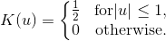
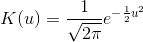
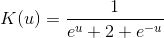
A kernel is a non-negative function normalized to area 1. The built-in kernels are centered at zero. Kernels are implemented by the Kernel class. The KernelDensity class provides several fields that represent common kernels. The available kernels are listed below:
Field | Equation | Chart |
|---|---|---|
 | ||
 | ||
 | ||
 | ||
 | ||
 | ||
 | ||
 | ||
 | ||
 |
Choose a Bandwidth
For untransformed fits, the bandwidth h is in observation units: each contribution is K((x-x_i)/h)/h. For the Gaussian kernel h is its component standard deviation. Other kernels use their declared argument scale; their component standard deviation need not equal h. Large widths can hide modes; small widths can amplify sampling noise. Supply a width with Fixed(Double, Kernel, Double), or select one with Automatic(KernelDensityBandwidthEstimator, Kernel, Double).
The KernelDensityBandwidthEstimator values below use normalized relative masses p_i, effective sample size n_eff = 1 / sum(p_i squared), and robust scale s = min(population SD, IQR/1.349), falling back to SD if IQR is zero. Without weights n_eff is the observation count. Quartiles use the Weibull convention described above. At least two positive-mass observations with positive spread are required.
Selector | Convention |
|---|---|
C(K) * s * n_eff^(-1/5), where C(K) depends on the normalized second-order kernel. For Gaussian C(K) = (4/3)^(1/5), approximately 1.059224. | |
0.9 * s * n_eff^(-1/5), retaining the existing rule-of-thumb convention. | |
1.059 * s * n_eff^(-1/5), retaining the existing constant and robust population-scale convention. | |
One-stage pilot-curvature plug-in for the built-in Gaussian kernel. Pilot width g = s * n_eff^(-1/9); select h = [1 / (2 sqrt(pi) n_eff R(f''_g))]^(1/5), where R(f''_g) is the integrated square of the Gaussian pilot density's second derivative. | |
Bounded leave-one-out least-squares cross-validation for the built-in Gaussian kernel. Select the best evaluated h for integral(f_h squared) - 2 sum_i p_i f_(-i,h)(x_i). The held-out density renormalizes all remaining masses. | |
Gaussian Sheather-Jones solve-the-equation selection, using pilot fourth- and sixth-derivative functionals. Root bracketing is automatic unless explicit bounds are supplied. |
The first three rules preserve Numerics.NET's existing formulas. Selector names alone do not guarantee agreement with another library: compare population versus sample SD, quartile definitions, scale fallbacks, kernel scaling, and whether a returned value is an absolute width or a covariance multiplier. The plug-in method here includes the pilot's diagonal terms without a finite-sample bias subtraction; it is not the Sheather-Jones selector. It can resolve structure missed by a normal-reference rule, but its pilot choice also affects the result.
KernelDensityEstimate plugInEstimate = KernelDensity.Fit(observations,
    KernelDensityOptions.Automatic(KernelDensityBandwidthEstimator.GaussianPlugIn), weights);
KernelDensityEstimate cvEstimate = KernelDensity.Fit(observations,
    KernelDensityOptions.CrossValidated(minimumBandwidth: .05, maximumBandwidth: 3), weights);
double selectedWidth = cvEstimate.UnadjustedBandwidth;
bool boundaryHit = cvEstimate.BandwidthSelectionAtBoundary;
// Inspect boundaryHit and the search bounds before accepting a constrained result.SheatherJones uses the Gaussian solve-the-equation selector. Pilots a = 1.24*s*n_eff^(-1/7) and b = 1.23*s*n_eff^(-1/9) estimate fourth- and sixth-derivative functionals. With alpha = 1.357*(psi4(a)/(-psi6(b)))^(1/7), solve h = [1/(2 sqrt(pi) n_eff psi4(alpha*h^(5/7)))]^(1/5). Functionals include diagonal pair terms and divide by the off-diagonal relative mass sum_i!=j p_i*p_j. Equal weights reduce to the n/(n-1) correction. Relative masses use the same effective sample size and robust scale as other selectors. The exact pair sums and population/weighted scale conventions can differ from binned implementations in other libraries.
Automatic selection brackets the equation near the normal-reference width and expands the bracket if necessary. SheatherJones(Double, Double, Double) supplies an explicit finite positive root bracket in fitting units before adjustment. An explicit bracket is never expanded: a bracket without a resolved root raises ArgumentException. Invalid derivative functionals or an unrepresentable root also raise an exception; no different selector is substituted. The fit reports the resolved bracket through its search metadata.
Vector<double> selectorData = Vector.Create(new double[] { -1, -.7, 0, .8, 2 });
KernelDensityEstimate sjEstimate = KernelDensity.Fit(selectorData,
    KernelDensityOptions.Automatic(KernelDensityBandwidthEstimator.SheatherJones));
double sjBandwidth = sjEstimate.UnadjustedBandwidth;
KernelDensityEstimate bracketedSj = KernelDensity.Fit(selectorData,
    KernelDensityOptions.SheatherJones(sjBandwidth / 2, sjBandwidth * 2));
double? bracketLower = bracketedSj.BandwidthSearchLowerBound;
double? bracketUpper = bracketedSj.BandwidthSearchUpperBound;Default cross-validation searches from 1/16 to 16 times the Gaussian normal-reference width, clamped to positive finite representable widths. Use CrossValidated(Double, Double, Double) for explicit bounds in observation units. The options' MinimumBandwidth and MaximumBandwidth report supplied bounds, or null when bounds were not supplied. The fit's BandwidthSearchLowerBound and BandwidthSearchUpperBound report resolved search bounds, or null for a method without a search. Bounds and UnadjustedBandwidth are before adjustment; the adjustment multiplies the selected width once afterward.
Cross-validation scans 65 logarithmically spaced widths and refines sampled minima and endpoint intervals with at most 64 golden-section steps per interval. The criterion can have several local minima; the best evaluated candidate is not a guarantee of the global optimum. BandwidthSelectionAtBoundary reports an endpoint selection. Check search bounds and repeated or rounded observations when this is true: duplicates can favor the smallest permitted width. No different selector is substituted silently. Relative weights are not replication counts; splitting a mass into repeated observations changes the leave-one-out problem even when a fixed-bandwidth density would be identical.
All three advanced selectors use exact Gaussian pair sums without binning or random subsampling. One-stage plug-in fitting costs O(n squared) time; cross-validation and Sheather-Jones cost O(E n squared), with E the number of criterion or functional evaluations. All use O(n) working storage. Use them for moderate samples; for large data, consider a representative fitting sample, a rule of thumb, or a supplied bandwidth. Other built-in or custom kernels with an advanced selector raise NotSupportedException.
EstimateBandwidth(Vector<Double>, Kernel, KernelDensityBandwidthEstimator) also accepts all six automatic selectors. Use the fitted API to inspect bandwidth-search bounds and boundary status or to supply observation weights. The legacy convenience methods SilvermanBandwidth(Vector<Double>), ScottBandwidth(Vector<Double>), and NormalReferenceBandwidth(Vector<Double>, Kernel) retain their existing results:
var bwRef = KernelDensity.NormalReferenceBandwidth(X, KernelDensity.GaussianKernel);
var bwSilverman = KernelDensity.EstimateBandwidth(X, KernelDensity.GaussianKernel,
KernelDensityBandwidthEstimator.Silverman);Computing Kernel Density Estimates
The Estimate method computes the estimated density for one value or a range of values. The scalar and batch overloads take up to 6 arguments. The first is a Vector<T> that contains the observations for which the density is to be estimated. The second argument is the kernel. The third argument is the value at which to evaluate the density. If a scalar is supplied, then the density at this value is returned. If a vector is supplied, then a vector of the densities at each value of the vector is returned.
The remaining arguments are all optional. The fourth argument is the bandwidth. If omitted, the bandwidth is estimated using the method specified by the KernelDensityBandwidthEstimator value passed as the fifth argument. The default is to use the normal reference bandwidth. The final argument is an adjustment factor for the bandwidth. This is useful when you want to specify the bandwidth as a fraction of an estimated bandwidth. The selection rule is ignored when a bandwidth is supplied explicitly; the adjustment factor always applies. Use named arguments to distinguish a query value, bandwidth and grid point count in the legacy overloads.
In the next example, we compute three different kernel density estimates. First, we use a Gaussian kernel and use the Silverman bandwidth we found earlier. Then we use an Epanechnikov kernel using Scott's rule to get the bandwidth. Finally, we use a tri-weight kernel and for the bandwidth we use half the normal reference bandwidth:
var density1 = KernelDensity.Estimate(X, KernelDensity.GaussianKernel, bandwidth: bwSilverman);
var density2 = KernelDensity.Estimate(X, KernelDensity.EpanechnikovKernel,
        bandwidthEstimator: KernelDensityBandwidthEstimator.Scott);
var density3 = KernelDensity.Estimate(X, KernelDensity.TriweightKernel,
bandwidthAdjustment: 0.5);The EstimateDistribution method performs the same operation, but returns a ContinuousDistribution that approximates the density on a finite grid. It normalizes trapezoidal cell masses over the padded sample range and constructs a piecewise distribution from the resulting cumulative probabilities. Its PDF is an approximation, and Gaussian or logistic tails outside the grid are omitted. The arguments to this method are mostly the same as before. The first argument is once again a vector of observations. The second argument is the kernel. The third through fifth arguments concern the bandwidth: the explicit bandwidth, the estimation method, and the adjustment, respectively.
The sixth argument specifies the number of points to use in the approximation of the density. If omitted, the larger of 50 and the number of inputs is used. At least three points are required. The seventh argument specifies how far past the lowest and highest observation the approximation should be computed, in units of the bandwidth. The default is 3.
In our last example, we estimate the density of our sample using a Gaussian kernel. The finite-grid approximation is returned as a probability distribution, which we can then use for other purposes, such as drawing more samples and computing expectation values:
var dist1 = KernelDensity.EstimateDistribution(X, KernelDensity.GaussianKernel);
var moreSamples = dist1.Sample(100);
var expectionValue = dist1.GetExpectationValue(x => Math.Exp(x));