Global Optimization

While traditional optimization methods such as gradient descent, Newton's method, and quasi-Newton methods are effective for finding local optima, they often struggle with complex problems that have multiple local optima. This is where global optimization methods come into play. Global optimization aims to find the absolute best solution across the entire search space, making it particularly valuable for problems where the landscape is rugged and filled with numerous peaks and valleys. By exploring the search space more broadly, global optimization techniques increase the likelihood of finding the true global optimum, rather than getting trapped in local optima.

One commonly used test function for evaluating optimization algorithms is the Rastrigin function. As you can see from the chart below, the function is highly multimodal, meaning it has a large number of local minima.

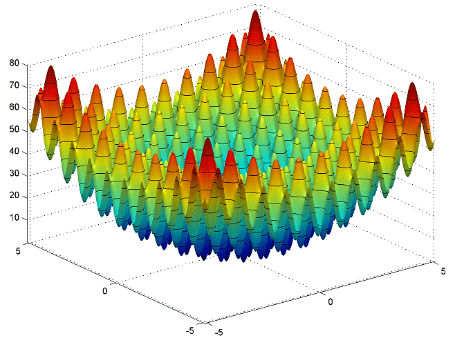The Rastrigin function is defined by the formula:

f (x) = A n + \sum_{i = 1}^{n} [x_{i}^{2} - A \cos (2 π x_{i})]

where $A$ is a constant (usually 10), $n$ is the dimensionality of the function. Despite its complexity, the global minimum is located at the origin, where the function value is zero. This makes the Rastrigin function a useful benchmark for testing the effectiveness of global optimization algorithms. We can implement the Rastrigin function as follows:

static double Rastrigin(Vector<double> x)
{
    const double A = 10;
    int n = x.Length;
    double sum = A * n;
    for (int i = 0; i < n; i++)
    {
        sum += x[i] * x[i] - A * Math.Cos(2 * Math.PI * x[i]);
    }
    return sum;
}

Visual Basic

Public shared function Rastrigin(x As Vector(Of double)) As double
    Const A = 10.0
    Dim n = x.Length
    Dim sum = A * n
    For i = 0 To n-1
        sum = sum + x(i) ^ 2 - A * Math.Cos(2 * Math.PI * x(i))
    Next
    Return sum
End Function

Visual Basic

No code example is currently available or this language may not be supported.

let Rastrigin (x: Vector<float>) =
    let A = 10.0
    let n = x.Length
    let initialSum = A * float n
    // Use direct iteration to avoid allocation of intermediate collections
    let mutable sum = 0.0
    for i = 0 to n - 1 do
        sum <- sum + (x.[i] * x.[i] - A * Math.Cos(2.0 * Math.PI * x.[i]))                    
    initialSum + sum

Numerics.NET provides a comprehensive suite of global optimization algorithms to address these challenges. These algorithms are designed to efficiently navigate complex search spaces and identify the best possible solutions for a wide range of optimization problems.

Available Algorithms

Numerics.NET includes several algorithms commonly used for global optimization, each with its own strengths and weaknesses:

Differential Evolution (DE): An evolutionary algorithm that optimizes a problem by iteratively trying to improve a candidate solution with regard to a given measure of quality. It uses simple mathematical operations to combine the positions of existing solutions to create new candidate solutions.
Particle Swarm Optimization (PSO): A population-based stochastic optimization technique inspired by the social behavior of birds flocking or fish schooling. Each particle in the swarm represents a candidate solution and moves through the search space based on its own experience and the experience of neighboring particles.
Covariance Matrix Adaptation Evolution Strategy (CMA-ES): An evolutionary algorithm that adapts the covariance matrix of the search distribution to improve the search efficiency. It is particularly effective for high-dimensional optimization problems.
Simulated Annealing (SA): A probabilistic technique that explores the search space by emulating the annealing process in metallurgy. It allows occasional uphill moves to escape local optima and gradually reduces the probability of such moves as the search progresses.

Global optimization is a powerful tool for solving complex problems that require finding the best possible solution within a defined search space. By leveraging advanced algorithms and techniques, Numerics.NET enables you to tackle a wide range of real-world challenges and achieve optimal outcomes.

Differential Evolution Optimizer

The DifferentialEvolutionOptimizer class implements the Differential Evolution (DE) algorithm. This population-based evolutionary finds the global optimum by maintaining a population of candidate solutions and generating new candidates through mutation and crossover operations.

The main advantage of the Differential Evolution algorithm is its robustness and ability to find global optima for non-convex, non-linear, and multimodal functions. It requires minimal tuning of control parameters and does not use gradient information, making it suitable for a wide range of optimization problems.

Basic Algorithm

The Differential Evolution algorithm works as follows:

Initialization: A population of candidate solutions is initialized randomly within the specified bounds.
Mutation: For each candidate solution, a mutant vector is generated by combining the positions of existing solutions using a weighted difference of randomly selected vectors.
Crossover: The mutant vector is combined with the current candidate solution to create a trial vector. This is done using either binomial or exponential crossover.
Selection: The trial vector is evaluated, and if it has a better objective value than the current candidate solution, it replaces the current solution in the population.
Iteration: The process of mutation, crossover, and selection is repeated for a specified number of iterations or until convergence criteria are met.

Configuration Parameters

The DifferentialEvolutionOptimizer class provides several properties and configuration parameters to control the optimization process:

CrossoverRate	The probability of crossover, which must be between 0 and 1. The default value is 0.9.
DifferentialWeight	The differential weight factor used in the mutation step, which must be between 0 and 2. The default value is 0.8.
MutationStrategy	The mutation strategy used to generate trial vectors. Different strategies offer different trade-offs between exploration and exploitation. The default is Best1Bin.
WeightDithering	The type of dithering applied to the differential weight to potentially improve convergence. The default is None.
DitheringRange	The range for uniform dithering when enabled. The default value is 0.1.
PopulationMultiplier	A multiplier for the population size. The total population is the number of free parameters times this value. The default value is 15.
StagnationLimit	The number of iterations without improvement before declaring stagnation. The default value is 20.

There are many mutation strategies to choose from. The following table lists the available strategies and their definitions:

Best1Bin	Uses the best solution with binomial crossover. The trial vector is generated by taking the best solution and adding the scaled difference between two randomly selected vectors. $v = best + F (r_{1} - r_{2})$
Best1Exp	Uses the best solution with exponential crossover. The trial vector is generated by taking the best solution and adding the scaled difference between two randomly selected vectors. $v = best + F (r_{1} - r_{2})$
Rand1Bin	Classical DE mutation with binomial crossover. The trial vector is generated by taking a random solution and adding the scaled difference between two other randomly selected vectors. $v = r_{1} + F (r_{2} - r_{3})$
Rand1Exp	Classical DE mutation with exponential crossover. The trial vector is generated by taking a random solution and adding the scaled difference between two other randomly selected vectors. $v = r_{1} + F (r_{2} - r_{3})$
Rand2Bin	Uses two difference vectors with binomial crossover. The trial vector is generated by taking a random solution and adding the scaled differences between two pairs of randomly selected vectors. $v = r_{1} + F (r_{2} - r_{3}) + F (r_{4} - r_{5})$
Rand2Exp	Uses two difference vectors with exponential crossover. The trial vector is generated by taking a random solution and adding the scaled differences between two pairs of randomly selected vectors. $v = r_{1} + F (r_{2} - r_{3}) + F (r_{4} - r_{5})$
Best2Bin	Uses the best solution and two differences with binomial crossover. The trial vector is generated by taking the best solution and adding the scaled differences between two pairs of randomly selected vectors. $v = best + F (r_{1} - r_{2}) + F (r_{3} - r_{4})$
Best2Exp	Uses the best solution and two differences with exponential crossover. The trial vector is generated by taking the best solution and adding the scaled differences between two pairs of randomly selected vectors. $v = best + F (r_{1} - r_{2}) + F (r_{3} - r_{4})$
RandToBest1Bin	Linear combination towards the best solution with binomial crossover. The trial vector is generated by taking a random solution and adding both the scaled difference between the best solution and itself and the scaled difference between two other random vectors. $v = r_{1} + F (best - r_{1}) + F (r_{2} - r_{3})$
RandToBest1Exp	Linear combination towards the best solution with exponential crossover. The trial vector is generated by taking a random solution and adding both the scaled difference between the best solution and itself and the scaled difference between two other random vectors. $v = r_{1} + F (best - r_{1}) + F (r_{2} - r_{3})$
CurrentToBest1Bin	Linear combination from the current solution towards the best solution with binomial crossover. The trial vector is generated by taking the current solution and adding both the scaled difference between the best and current solutions and the scaled difference between two random vectors. $v = current + F (best - current) + F (r_{1} - r_{2})$
CurrentToBest1Exp	Linear combination from the current solution towards the best solution with exponential crossover. The trial vector is generated by taking the current solution and adding both the scaled difference between the best and current solutions and the scaled difference between two random vectors. $v = current + F (best - current) + F (r_{1} - r_{2})$

The mutation strategies are built on two key elements: how the base solution is chosen and how its components are combined with others to form a new trial solution. The first element influences whether the search is driven toward promising regions by exploiting the best-known information or whether it maintains exploration by injecting randomness. The second element determines the manner in which solution components are exchanged—either independently for each dimension or as contiguous segments—thus affecting the preservation of beneficial structural patterns.

In the "best" variant, the mutation uses the best candidate from the population as the base, quickly steering the search toward promising areas but potentially risking premature convergence. In contrast, the "rand" variant picks the base completely at random from the population, which preserves diversity and promotes broader exploration at the cost of slower convergence. The "current-to-best" variant starts with the current candidate and nudges it toward the best candidate, thereby balancing local refinement with global guidance. This can speed up convergence while still retaining some individuality. Similarly, the "rand-to-best" variant begins with a randomly selected candidate and shifts it toward the best candidate, blending random exploration with directed improvement. These approaches aim to combine the benefits of both extremes, providing a flexible trade-off between convergence speed and maintaining diversity.

Binomial crossover treats each dimension independently, randomly selecting each component from either the mutant or the target solution, which leads to a highly varied mix of genes across all dimensions. In contrast, exponential crossover starts at a random index and then takes a continuous block of components from the mutant before switching to the target solution for the remaining dimensions. This contiguous selection can help preserve beneficial patterns or structures that span several dimensions, making exponential crossover more effective when neighboring variables are correlated.

The choice between binomial and exponential crossover can impact the algorithm's exploration vs exploitation behavior. Binomial crossover typically provides better exploration by allowing changes throughout the vector, while exponential crossover tends to focus changes in specific regions, potentially enabling better local exploitation.

The default strategy is Best1Bin. It generally provides good performance across a wide range of problems. strategy, which is a good starting point for most problems.

Code Example

Let's explore how to use the DifferentialEvolutionOptimizer class to optimize a function through a step-by-step guide. We'll use the Rastrigin function as our example.

Define the search space

Specify the dimensions and bounds of your optimization problem:

// Set the dimensionality of the problem
int dimensions = 10;

// Define the search space bounds
var lowerBounds = Vector.CreateConstant(dimensions, -5.12);
var upperBounds = Vector.CreateConstant(dimensions, 5.2345);

Visual Basic

' Set the dimensionality of the problem
Dim dimensions = 10

' Define the search space bounds
Dim lowerBounds = Vector.CreateConstant(dimensions, -5.12)
Dim upperBounds = Vector.CreateConstant(dimensions, 5.2345)

Visual Basic

No code example is currently available or this language may not be supported.

// Set the dimensionality of the problem
let dimensions = 10

// Define the search space bounds
let lowerBounds = Vector.CreateConstant(dimensions, -5.12)
let upperBounds = Vector.CreateConstant(dimensions, 5.2345)

Create and configure the optimizer

There are two ways to instantiate the optimizer. One is to provide the basic settings in the constructor:

var optimizer = new DifferentialEvolutionOptimizer(
    objectiveFunction: Rastrigin,
    lowerBounds: lowerBounds,
    upperBounds: upperBounds
);

Visual Basic

Dim optimizer = New DifferentialEvolutionOptimizer(
    AddressOf Rastrigin, lowerBounds, upperBounds)

Visual Basic

No code example is currently available or this language may not be supported.

let optimizer = new DifferentialEvolutionOptimizer(
    objectiveFunction=Rastrigin,
    lowerBounds=lowerBounds,
    upperBounds=upperBounds)

Another is to call the default constructor and set all properties afterwards:

var optimizer2 = new DifferentialEvolutionOptimizer() {
    ObjectiveFunction = Rastrigin,
    LowerBounds = lowerBounds,
    UpperBounds = upperBounds
};

Visual Basic

Dim optimizer2 = New DifferentialEvolutionOptimizer()
optimizer2.ObjectiveFunction = AddressOf Rastrigin
optimizer2.LowerBounds = lowerBounds
optimizer2.UpperBounds = upperBounds

Visual Basic

No code example is currently available or this language may not be supported.

let optimizer2 = new DifferentialEvolutionOptimizer()
optimizer2.ObjectiveFunction <- Rastrigin
optimizer2.LowerBounds <- lowerBounds
optimizer2.UpperBounds <- upperBounds

If desired, you can set various properties to fine-tune the algorithm's execution:

// Adjust the crossover probability (default is 0.9)
optimizer.CrossoverRate = 0.8;

// Set the differential weight factor (default is 0.8)
optimizer.DifferentialWeight = 0.7;

// Choose a mutation strategy (default is Best1Bin)
optimizer.MutationStrategy = DifferentialEvolutionStrategy.Best1Bin;

// Enable weight dithering for potentially better convergence
optimizer.WeightDithering = DifferentialWeightDithering.Uniform;
optimizer.DitheringRange = 0.2;

// Adjust population size (default multiplier is 15)
optimizer.PopulationMultiplier = 20;

// Set stagnation detection (default is 20 iterations)
optimizer.StagnationLimit = 30;

Visual Basic

' Adjust the crossover probability (default is 0.9)
optimizer.CrossoverRate = 0.8

' Set the differential weight factor (default is 0.8)
optimizer.DifferentialWeight = 0.7

' Choose a mutation strategy (default is Best1Bin)
optimizer.MutationStrategy = DifferentialEvolutionStrategy.Best1Bin

' Enable weight dithering for potentially better convergence
optimizer.WeightDithering = DifferentialWeightDithering.Uniform
optimizer.DitheringRange = 0.2

' Adjust population size (default multiplier is 15)
optimizer.PopulationMultiplier = 20

' Set stagnation detection (default is 20 iterations)
optimizer.StagnationLimit = 30

Visual Basic

No code example is currently available or this language may not be supported.

// Adjust the crossover probability (default is 0.9)
optimizer.CrossoverRate <- 0.8

// Set the differential weight factor (default is 0.8)
optimizer.DifferentialWeight <- 0.7

// Choose a mutation strategy (default is Best1Bin)
optimizer.MutationStrategy <- DifferentialEvolutionStrategy.Best1Bin

// Enable weight dithering for potentially better convergence
optimizer.WeightDithering <- DifferentialWeightDithering.Uniform
optimizer.DitheringRange <- 0.2

// Adjust population size (default multiplier is 15)
optimizer.PopulationMultiplier <- 20

// Set stagnation detection (default is 20 iterations)
optimizer.StagnationLimit <- 30

Run the optimization

Execute the optimization process:

optimizer.FindMinimum();

Visual Basic

optimizer.FindMinimum()

Visual Basic

No code example is currently available or this language may not be supported.

let result = optimizer.FindMinimum()

Retrieve and analyze the results

Access the optimization results:

// Get the optimum solution vector
var solution = optimizer.Extremum;

// Get the function value at the optimum
double objectiveValue = optimizer.ValueAtExtremum;

// Check if the optimization converged successfully
bool converged = optimizer.Status == AlgorithmStatus.Converged;

// Get the number of function evaluations performed
int evaluations = optimizer.EvaluationsNeeded;

// Display the results
Console.WriteLine("Optimization completed:");
Console.WriteLine($"- Converged: {converged}");
Console.WriteLine($"- Function evaluations: {evaluations}");
Console.WriteLine($"- Optimal solution: {solution}");
Console.WriteLine($"- Objective value at optimum: {objectiveValue}");

Visual Basic

' Get the optimum solution vector
Dim solution = optimizer.Extremum

' Get the function value at the optimum
Dim objectiveValue = optimizer.ValueAtExtremum

' Check if the optimization converged successfully
Dim converged = optimizer.Status = AlgorithmStatus.Converged

' Get the number of function evaluations performed
Dim evaluations = optimizer.EvaluationsNeeded

' Display the results
Console.WriteLine("Optimization completed:")
Console.WriteLine($"- Converged: {converged}")
Console.WriteLine($"- Function evaluations: {evaluations}")
Console.WriteLine($"- Optimal solution: {solution}")
Console.WriteLine($"- Objective value at optimum: {objectiveValue}")

Visual Basic

No code example is currently available or this language may not be supported.

// Get the optimum solution vector
let solution = optimizer.Extremum

// Get the function value at the optimum
let objectiveValue = optimizer.ValueAtExtremum

// Check if the optimization converged successfully
let converged = optimizer.Status = AlgorithmStatus.Converged

// Get the number of function evaluations performed
let evaluations = optimizer.EvaluationsNeeded

// Display the results
printfn "Optimization completed:"
printfn "- Converged: %b" converged
printfn "- Function evaluations: %d" evaluations
printfn "- Optimal solution: %O" solution
printfn "- Objective value at optimum: %f" objectiveValue

By following these steps, you can apply the Differential Evolution optimizer to a variety of optimization problems. You can experiment with different parameter settings to find the most effective configuration for your specific problem.

For challenging problems, it's often helpful to try different mutation strategies and parameter values. The Best1Bin strategy typically provides fast convergence but might get trapped in local optima, while Rand1Bin offers more exploration at the cost of slower convergence.

Particle Swarm Optimization

The ParticleSwarmOptimizer class implements the Particle Swarm Optimization (PSO) algorithm for multi-dimensional optimization. PSO is a population-based stochastic optimization technique inspired by the social behavior of bird flocking or fish schooling. Each particle in the swarm represents a candidate solution and moves through the search space according to its own experience and the experience of neighboring particles.

Basic Algorithm

The Particle Swarm Optimization algorithm works as follows:

Initialization: A population of particles is initialized with random positions and velocities within the specified bounds.
Evaluation: Each particle's position is evaluated using the objective function to determine its fitness.
Update Personal Best: Each particle updates its personal best position if the current position is better.
Update Neighborhood Best: The best position among the particle's neighborhood is updated based on the topology.
Update Velocity and Position: Each particle's velocity is updated based on its inertia, cognitive component (personal best), and social component (neighborhood best). The particle's position is then updated based on the new velocity.
Iteration: The process of evaluation, updating personal best, updating neighborhood best, and updating velocity and position is repeated for a specified number of iterations or until convergence criteria are met.

Configuration Parameters

The ParticleSwarmOptimizer class provides several properties and configuration parameters to control the optimization process:

ConstrictionFactor	The constriction factor controls the impact of previous velocities. The default value is 0.729 which is optimal in many cases.
CognitiveCoefficient	The cognitive coefficient (c1) controls the influence of personal best positions. The default value is 1.49445.
SocialCoefficient	The social coefficient (c2) controls the influence of the global best position. The default value is 1.49445.
MaxVelocity	The maximum velocity factor as a proportion of the search space. The default value is 4.0.
Topology	The topology of the particle swarm, which defines the neighborhood relationships between particles. The default is Global.
PopulationMultiplier	A multiplier for the population size. The total population is the number of free parameters times this value. The default value is 10.
StagnationLimit	The number of iterations without improvement before declaring stagnation. The default value is 20.

The ConstrictionFactor is a crucial parameter that helps control the convergence characteristics of the swarm. Typical values are between 0.4 and 0.9. Lower values favor local search while higher values favor global exploration. The default value of 0.729 is derived from theoretical analysis and provides good balance between exploration and exploitation. For highly multimodal problems, consider increasing it to 0.8-0.9 to maintain more exploration capability. For simple unimodal problems, you can reduce it to 0.4-0.6 for faster convergence.

The CognitiveCoefficient and SocialCoefficient work together to balance individual and collective behavior. The default values (≈1.49445) are derived from stability analysis and work well for most problems. Setting c1 > c2 emphasizes exploration of individual particles' experiences, while c2 > c1 promotes exploitation of social knowledge. For problems with many local optima, try increasing c1 relative to c2 (e.g., c1=1.7, c2=1.3) to maintain diversity.

The MaxVelocity prevents particles from taking excessively large steps, which could lead to erratic behavior. The default value of 4.0 means particles can move up to 4 times the width of the search space in a single step. For smooth, well-behaved functions, you might reduce this to 1.0-2.0 for more controlled movement. For rugged landscapes with distant optima, larger values (5.0-10.0) might help particles escape local minima.

The PopulationMultiplier determines how many particles to use relative to the problem dimension. The default value of 10 means a 3-dimensional problem will use 30 particles. For simple problems, you might reduce this to 5-7 for efficiency. For complex, highly multimodal problems, consider increasing it to 15-20 to improve exploration, though this increases computational cost proportionally.

The StagnationLimit helps prevent wasteful computation when the swarm has converged or is stuck. The default value of 20 iterations is conservative. For expensive objective functions, you might reduce this to 10-15 to terminate earlier. For problems where the optimum is hard to find or where small improvements are valuable, consider increasing it to 30-50. If the algorithm frequently hits this limit, you might need to adjust other parameters to improve exploration.

The Topology defines the neighborhood relationships between particles in the swarm. The topology determines how particles influence each other during the optimization process. Different topologies can affect the convergence behavior and performance of the PSO algorithm.

You create a topology by calling one of the static methods of the ParticleSwarmTopology structure. The following options are available:

Global	In the global topology, each particle is influenced by every other particle in the swarm. This topology promotes global exploration and is suitable for problems where a broad search of the solution space is needed.
Ring	In the ring topology, each particle is influenced by its neighbors in a ring structure. The number of neighbors on each side of a particle can be specified. The default is 1. This topology promotes local exploration and can help maintain diversity in the swarm.
VonNeumann	In the Von Neumann topology, each particle is influenced by its neighbors in a grid structure. This topology promotes local exploration and can help maintain diversity in the swarm.
Random	In the random topology, each particle is influenced by a random subset of particles. The size of the neighborhood can be specified as well as how often (in iterations) the connections should be updated with new random values. This topology provides a balance between global and local exploration.

Code Example

Let's explore how to use the ParticleSwarmOptimizer class to optimize a function through a step-by-step guide. We'll use the Rastrigin function as our example.

Define the search space

Specify the dimensions and bounds of your optimization problem:

// Set the dimensionality of the problem
int dimensions = 10;

// Define the search space bounds
var lowerBounds = Vector.CreateConstant(dimensions, -5.12);
var upperBounds = Vector.CreateConstant(dimensions, 5.2345);

Visual Basic

' Set the dimensionality of the problem
Dim dimensions = 10

' Define the search space bounds
Dim lowerBounds = Vector.CreateConstant(dimensions, -5.12)
Dim upperBounds = Vector.CreateConstant(dimensions, 5.2345)

Visual Basic

No code example is currently available or this language may not be supported.

// Set the dimensionality of the problem
let dimensions = 10

// Define the search space bounds
let lowerBounds = Vector.CreateConstant(dimensions, -5.12)
let upperBounds = Vector.CreateConstant(dimensions, 5.2345)

Create and configure the optimizer

Instantiate the Particle Swarm optimizer with the objective function and bounds:

There are two ways to instantiate the optimizer. One is to provide the basic settings in the constructor:

var optimizer = new ParticleSwarmOptimizer(
    objectiveFunction: Rastrigin,
    lowerBounds: lowerBounds,
    upperBounds: upperBounds
);

Visual Basic

Dim optimizer = New ParticleSwarmOptimizer(
    AddressOf Rastrigin, lowerBounds, upperBounds)

Visual Basic

No code example is currently available or this language may not be supported.

let optimizer = new ParticleSwarmOptimizer(
    objectiveFunction=Rastrigin,
    lowerBounds=lowerBounds,
    upperBounds=upperBounds)

Another is to call the default constructor and set all properties afterwards:

var optimizer2 = new ParticleSwarmOptimizer() {
    ObjectiveFunction = Rastrigin,
    LowerBounds = lowerBounds,
    UpperBounds = upperBounds
};

Visual Basic

Dim optimizer2 = New ParticleSwarmOptimizer()
optimizer2.ObjectiveFunction = AddressOf Rastrigin
optimizer2.LowerBounds = lowerBounds
optimizer2.UpperBounds = upperBounds

Visual Basic

No code example is currently available or this language may not be supported.

let optimizer2 = new ParticleSwarmOptimizer()
optimizer2.ObjectiveFunction <- Rastrigin
optimizer2.LowerBounds <- lowerBounds
optimizer2.UpperBounds <- upperBounds

If needed, configure the optimizer by adjusting its properties to fine-tune the algorithm:

// Set constriction factor  
optimizer.ConstrictionFactor = 0.729;

// Set cognitive coefficient  
optimizer.CognitiveCoefficient = 1.49445;

// Set social coefficient  
optimizer.SocialCoefficient = 1.49445;

// Set maximum velocity  
optimizer.MaxVelocity = 4.0;

// Set topology to Ring with 2 neighbors on each side
optimizer.Topology = ParticleSwarmTopology.Ring(2);

// Set population multiplier  
optimizer.PopulationMultiplier = 10;

// Set stagnation limit  
optimizer.StagnationLimit = 20;

Visual Basic

' Set constriction factor  
optimizer.ConstrictionFactor = 0.729

' Set cognitive coefficient  
optimizer.CognitiveCoefficient = 1.49445

' Set social coefficient  
optimizer.SocialCoefficient = 1.49445

' Set maximum velocity  
optimizer.MaxVelocity = 4.0

' Set topology to Ring with 2 neighbors on each side
optimizer.Topology = ParticleSwarmTopology.Ring(2)

' Set population multiplier  
optimizer.PopulationMultiplier = 10

' Set stagnation limit  
optimizer.StagnationLimit = 20

Visual Basic

No code example is currently available or this language may not be supported.

// Set constriction factor  
optimizer.ConstrictionFactor <- 0.729

// Set cognitive coefficient  
optimizer.CognitiveCoefficient <- 1.49445

// Set social coefficient  
optimizer.SocialCoefficient <- 1.49445

// Set maximum velocity  
optimizer.MaxVelocity <- 4.0

// Set topology to Ring with 2 neighbors on each side
optimizer.Topology <- ParticleSwarmTopology.Ring(2)

// Set population multiplier  
optimizer.PopulationMultiplier <- 10

// Set stagnation limit  
optimizer.StagnationLimit <- 20

Run the optimization

Execute the optimization process:

optimizer.FindMinimum();

Visual Basic

optimizer.FindMinimum()

Visual Basic

No code example is currently available or this language may not be supported.

let result = optimizer.FindMinimum()

Retrieve and analyze the results

Access the optimization results:

// Get the optimum solution vector
var solution = optimizer.Extremum;

// Get the function value at the optimum
double objectiveValue = optimizer.ValueAtExtremum;

// Check if the optimization converged successfully
bool converged = optimizer.Status == AlgorithmStatus.Converged;

// Get the number of function evaluations performed
int evaluations = optimizer.EvaluationsNeeded;

// Display the results
Console.WriteLine("Optimization completed:");
Console.WriteLine($"- Converged: {converged}");
Console.WriteLine($"- Function evaluations: {evaluations}");
Console.WriteLine($"- Optimal solution: {solution}");
Console.WriteLine($"- Objective value at optimum: {objectiveValue}");

Visual Basic

' Get the optimum solution vector
Dim solution = optimizer.Extremum

' Get the function value at the optimum
Dim objectiveValue = optimizer.ValueAtExtremum

' Check if the optimization converged successfully
Dim converged = optimizer.Status = AlgorithmStatus.Converged

' Get the number of function evaluations performed
Dim evaluations = optimizer.EvaluationsNeeded

' Display the results
Console.WriteLine("Optimization completed:")
Console.WriteLine($"- Converged: {converged}")
Console.WriteLine($"- Function evaluations: {evaluations}")
Console.WriteLine($"- Optimal solution: {solution}")
Console.WriteLine($"- Objective value at optimum: {objectiveValue}")

Visual Basic

No code example is currently available or this language may not be supported.

// Get the optimum solution vector
let solution = optimizer.Extremum

// Get the function value at the optimum
let objectiveValue = optimizer.ValueAtExtremum

// Check if the optimization converged successfully
let converged = optimizer.Status = AlgorithmStatus.Converged

// Get the number of function evaluations performed
let evaluations = optimizer.EvaluationsNeeded

// Display the results
printfn "Optimization completed:"
printfn "- Converged: %b" converged
printfn "- Function evaluations: %d" evaluations
printfn "- Optimal solution: %O" solution
printfn "- Objective value at optimum: %f" objectiveValue

By following these steps, you can apply the Particle Swarm Optimization algorithm to a variety of optimization problems. Experiment with different topologies and parameter settings to find the most effective configuration for your specific problem.

For challenging multimodal problems like Rastrigin, it's often beneficial to try different topologies. The Global topology provides faster convergence but might get trapped in local optima, while Ring or Von Neumann topologies allow for more exploration of the search space at the cost of slower convergence.

CMA Evolution Strategy Optimizer

The CMAEvolutionStrategyOptimizer class implements the Covariance Matrix Adaptation Evolution Strategy (CMA-ES) algorithm for multi-dimensional optimization. CMA-ES is a stochastic, derivative-free optimization algorithm designed for difficult optimization problems in continuous domains. It adapts the full covariance matrix of a normal search distribution, allowing it to efficiently navigate complex search spaces.

Basic Algorithm

The CMA-ES algorithm works as follows:

Initialization: A population of candidate solutions is initialized with random positions within the specified bounds.
Evaluation: Each candidate solution is evaluated using the objective function to determine its fitness.
Selection and Recombination: The best solutions are selected, and a new mean is calculated by weighted recombination of the selected solutions.
Update Evolution Paths: The evolution paths for the covariance matrix and step size are updated based on the new mean.
Adapt Covariance Matrix: The covariance matrix is updated using the evolution paths and the selected solutions.
Update Step Size: The step size is updated based on the evolution path for the step size.
Iteration: The process of evaluation, selection and recombination, updating evolution paths, adapting the covariance matrix, and updating the step size is repeated for a specified number of iterations or until convergence criteria are met.

Configuration Parameters

The CMAEvolutionStrategyOptimizer class provides several properties and configuration parameters to control the optimization process:

InitialStepSize	The initial step size (σ) for the search distribution. The default value is 0.5.
UseActiveCMA	A boolean value indicating whether to use active CMA, which includes negative updates to the covariance matrix. The default value is false.
UseDiagonalCovarianceMatrix	A boolean value indicating whether to use a diagonal covariance matrix instead of a full covariance matrix. The default value is false.
BoundaryHandling	The boundary handling strategy for the optimizer. Options include None, Reflect, and Resample.

The CMA-ES algorithm's behavior can be fine-tuned through its properties to optimize performance for different types of problems:

The initial step size (InitialStepSize) is crucial for the algorithm's exploration behavior. A larger step size promotes exploration of the search space but may slow convergence, while a smaller step size focuses on local refinement but risks getting trapped in local optima. As a rule of thumb, set it to about 1/3 of the expected distance to the optimum.

Active CMA (UseActiveCMA) can significantly improve the convergence speed on many problems by actively punishing undesirable directions in the search space. Enable this option when dealing with difficult problems where standard CMA-ES shows slow progress. However, it may be less stable on noisy problems.

Using a diagonal covariance matrix (UseDiagonalCovarianceMatrix) reduces computational complexity from O(n²) to O(n) and memory requirements from O(n²) to O(n), where n is the problem dimension. Enable this option for high-dimensional problems (n > 100) or when variables are known to be largely independent. However, it reduces the algorithm's ability to learn variable dependencies.

The boundary handling strategy (BoundaryHandling) determines how the algorithm deals with solutions that violate box constraints. Use Reflect for problems where the optimum is likely near the boundaries, Resample when maintaining strictly feasible solutions is critical, and None when soft constraints are acceptable or when the optimum is likely far from the boundaries.

Code Example

Let's explore how to use the CMAEvolutionStrategyOptimizer class to optimize a function through a step-by-step guide. We'll use the Rastrigin function as our example.

Define the search space

Specify the dimensions, initial guess, and bounds of your optimization problem:

// Set the dimensionality of the problem
int dimensions = 10;

// Define an initial guess for the solution
var initialGuess = 5.0 * Vector.CreateRandom(dimensions);

Visual Basic

' Set the dimensionality of the problem
Dim dimensions = 10

' Define an initial guess for the solution
Dim initialGuess = 5.0 * Vector.CreateRandom(dimensions)

Visual Basic

No code example is currently available or this language may not be supported.

// Set the dimensionality of the problem
let dimensions = 10

// Define an initial guess for the solution
let initialGuess = 5.0 * Vector.CreateRandom(dimensions)

Create and configure the optimizer

Instantiate the CMA-ES optimizer with the objective function and parameters:

var optimizer = new CMAEvolutionStrategyOptimizer(
    objectiveFunction: Rastrigin,
    initialGuess: initialGuess
);

Visual Basic

Dim optimizer = New CMAEvolutionStrategyOptimizer(
    AddressOf Rastrigin, initialGuess)

Visual Basic

No code example is currently available or this language may not be supported.

let optimizer = new CMAEvolutionStrategyOptimizer(
    Rastrigin, initialGuess)

You can also customize additional properties to fine-tune the algorithm:

// Set the initial step size for the search distribution
optimizer.InitialStepSize = 0.5;

// Enable active CMA for faster convergence
optimizer.UseActiveCMA = true;

// Use a full covariance matrix. Set to true for high-dimensional problems
optimizer.UseDiagonalCovarianceMatrix = false;

// Set boundary handling to reflect
optimizer.BoundaryHandling = BoxConstraintHandlingMethod.Reflect;

// Set the maximum number of iterations
optimizer.MaxIterations = 1000;

Visual Basic

' Set the initial step size for the search distribution
optimizer.InitialStepSize = 0.5

' Enable active CMA for faster convergence
optimizer.UseActiveCMA = true

' Use a full covariance matrix. Set to true for high-dimensional problems
optimizer.UseDiagonalCovarianceMatrix = false

' Set boundary handling to reflect
optimizer.BoundaryHandling = BoxConstraintHandlingMethod.Reflect

' Set the maximum number of iterations
optimizer.MaxIterations = 1000

Visual Basic

No code example is currently available or this language may not be supported.

// Set the initial step size for the search distribution
optimizer.InitialStepSize <- 0.5

// Enable active CMA for faster convergence
optimizer.UseActiveCMA <- true

// Use a full covariance matrix. Set to true for high-dimensional problems
optimizer.UseDiagonalCovarianceMatrix <- false

// Set boundary handling to reflect
optimizer.BoundaryHandling <- BoxConstraintHandlingMethod.Reflect

// Set the maximum number of iterations
optimizer.MaxIterations <- 1000

Run the optimization

Execute the optimization process:

optimizer.FindMinimum();

Visual Basic

optimizer.FindMinimum()

Visual Basic

No code example is currently available or this language may not be supported.

let result = optimizer.FindMinimum()

Retrieve and analyze the results

Access the optimization results:

// Get the optimum solution vector
var solution = optimizer.Extremum;

// Get the function value at the optimum
double objectiveValue = optimizer.ValueAtExtremum;

// Check if the optimization converged successfully
bool converged = optimizer.Status == AlgorithmStatus.Converged;

// Get the number of function evaluations performed
int evaluations = optimizer.EvaluationsNeeded;

// Display the results
Console.WriteLine("Optimization completed:");
Console.WriteLine($"- Converged: {converged}");
Console.WriteLine($"- Function evaluations: {evaluations}");
Console.WriteLine($"- Optimal solution: {solution}");
Console.WriteLine($"- Objective value at optimum: {objectiveValue}");

Visual Basic

' Get the optimum solution vector
Dim solution = optimizer.Extremum

' Get the function value at the optimum
Dim objectiveValue = optimizer.ValueAtExtremum

' Check if the optimization converged successfully
Dim converged = optimizer.Status = AlgorithmStatus.Converged

' Get the number of function evaluations performed
Dim evaluations = optimizer.EvaluationsNeeded

' Display the results
Console.WriteLine("Optimization completed:")
Console.WriteLine($"- Converged: {converged}")
Console.WriteLine($"- Function evaluations: {evaluations}")
Console.WriteLine($"- Optimal solution: {solution}")
Console.WriteLine($"- Objective value at optimum: {objectiveValue}")

Visual Basic

No code example is currently available or this language may not be supported.

// Get the optimum solution vector
let solution = optimizer.Extremum

// Get the function value at the optimum
let objectiveValue = optimizer.ValueAtExtremum

// Check if the optimization converged successfully
let converged = optimizer.Status = AlgorithmStatus.Converged

// Get the number of function evaluations performed
let evaluations = optimizer.EvaluationsNeeded

// Display the results
printfn "Optimization completed:"
printfn "- Converged: %b" converged
printfn "- Function evaluations: %d" evaluations
printfn "- Optimal solution: %O" solution
printfn "- Objective value at optimum: %f" objectiveValue

By following these steps, you can apply the CMA-ES optimizer to a variety of complex optimization problems. This algorithm is particularly effective for high-dimensional problems and functions with rugged landscapes.

For challenging problems, consider experimenting with different parameter settings, especially the initial step size and whether to use active CMA or diagonal covariance matrices. The active CMA can improve performance by including negative updates to the covariance matrix, while using diagonal matrices can speed up computation for very high-dimensional problems at the cost of some optimization power.

Simulated Annealing Optimizer

The SimulatedAnnealingOptimizer class implements the Simulated Annealing algorithm for multi-dimensional optimization. Simulated Annealing is a probabilistic optimization technique inspired by the annealing process in metallurgy. The algorithm allows accepting worse solutions with a probability that decreases as the temperature decreases, enabling escape from local optima.

Basic Algorithm

The Simulated Annealing algorithm works as follows:

Initialization: The initial solution is generated randomly within the specified bounds, and the initial temperature is set.
Evaluation: The current solution is evaluated using the objective function to determine its fitness.
Generate Neighbor: A new candidate solution is generated in the neighborhood of the current solution.
Acceptance Criterion: The new solution is accepted based on the Metropolis criterion, which allows worse solutions to be accepted with a probability that decreases as the temperature decreases.
Update Temperature: The temperature is updated according to the cooling schedule.
Iteration: The process of evaluation, generating a neighbor, applying the acceptance criterion, and updating the temperature is repeated for a specified number of iterations or until convergence criteria are met.

Configuration Parameters

The SimulatedAnnealingOptimizer class provides several properties and configuration parameters to control the optimization process:

InitialTemperature	The initial temperature for the annealing process. The default value is 100.0.
MinTemperature	The minimum temperature at which to stop the annealing process. The default value is 1e-8.
CoolingRate	The rate at which the temperature decreases, a value between 0 and 1. The default value is 0.95.
IterationsPerTemperatureLevel	The number of iterations to perform at each temperature level. The default value is 100.
NeighborhoodSize	The size of the neighborhood for generating new solutions, a value between 0 and 1. The default value is 0.1.
StagnationLimit	The maximum number of iterations without improvement before terminating. The default value is 1000.

These parameters work together to control the balance between exploration and exploitation in the simulated annealing process:

InitialTemperature determines how likely the algorithm is to accept worse solutions at the start. Higher values (500-1000) promote more exploration of the search space, while lower values (10-50) focus more on local improvements. For complex multimodal problems, use higher temperatures to avoid getting trapped in local optima early. For simpler problems with fewer local optima, lower temperatures may suffice.

MinTemperature acts as a stopping criterion and determines when the algorithm switches to pure hill climbing. The default of 1e-8 works well for most problems. Increase this value (e.g., 1e-4) to terminate earlier with potentially good-enough solutions, or decrease it (e.g., 1e-12) to allow more thorough but slower optimization.

CoolingRate controls how quickly the temperature decreases and thus how fast the algorithm transitions from exploration to exploitation. Values closer to 1.0 (e.g., 0.99) result in slower cooling and more thorough exploration but require more iterations. Values around 0.8-0.9 provide faster convergence but may miss global optima. For complex problems, use slower cooling rates (0.95-0.99).

IterationsPerTemperatureLevel defines how thoroughly each temperature level is explored. Higher values allow better exploration at each temperature but increase computation time. For high-dimensional problems (n > 10), consider using at least 100n iterations. For simpler problems, 50-100 iterations per level may be sufficient.

NeighborhoodSize determines how far the algorithm looks for new solutions relative to the current one. Larger values (0.2-0.5) enable broader jumps and are useful early in optimization, while smaller values (0.01-0.1) focus on local refinement. Consider decreasing this value as the temperature drops to focus more on local optimization.

StagnationLimit prevents excessive computation when no improvements are found. For simple problems, 500-1000 iterations is usually sufficient. For complex problems with many local optima, consider higher values (2000-5000) to allow more thorough exploration. If the algorithm frequently hits this limit, consider increasing the initial temperature or cooling rate to promote more exploration.

Code Example

Let's explore how to use the SimulatedAnnealingOptimizer class to optimize a function through a step-by-step guide. We'll use the Rastrigin function as our example.

Define the search space

Specify the dimensions and bounds of your optimization problem:

// Set the dimensionality of the problem
int dimensions = 10;

// Define the search space bounds
var lowerBounds = Vector.CreateConstant(dimensions, -5.12);
var upperBounds = Vector.CreateConstant(dimensions, 5.2345);

Visual Basic

' Set the dimensionality of the problem
Dim dimensions = 10

' Define the search space bounds
Dim lowerBounds = Vector.CreateConstant(dimensions, -5.12)
Dim upperBounds = Vector.CreateConstant(dimensions, 5.2345)

Visual Basic

No code example is currently available or this language may not be supported.

// Set the dimensionality of the problem
let dimensions = 10

// Define the search space bounds
let lowerBounds = Vector.CreateConstant(dimensions, -5.12)
let upperBounds = Vector.CreateConstant(dimensions, 5.2345)

Create and configure the optimizer

There are two ways to instantiate the optimizer. One is to provide the basic settings in the constructor:

var optimizer = new SimulatedAnnealingOptimizer(
    objectiveFunction: Rastrigin,
    lowerBounds: lowerBounds,
    upperBounds: upperBounds
);

Visual Basic

Dim optimizer = New SimulatedAnnealingOptimizer(
    AddressOf Rastrigin, lowerBounds, upperBounds)

Visual Basic

No code example is currently available or this language may not be supported.

let optimizer = new SimulatedAnnealingOptimizer(
    objectiveFunction=Rastrigin,
    lowerBounds=lowerBounds,
    upperBounds=upperBounds)

Another is to call the default constructor and set all properties afterwards:

var optimizer2 = new SimulatedAnnealingOptimizer() {
    ObjectiveFunction = Rastrigin,
    LowerBounds = lowerBounds,
    UpperBounds = upperBounds
};

Visual Basic

Dim optimizer2 = New SimulatedAnnealingOptimizer()
optimizer2.ObjectiveFunction = AddressOf Rastrigin
optimizer2.LowerBounds = lowerBounds
optimizer2.UpperBounds = upperBounds

Visual Basic

No code example is currently available or this language may not be supported.

let optimizer2 = new SimulatedAnnealingOptimizer()
optimizer2.ObjectiveFunction <- Rastrigin
optimizer2.LowerBounds <- lowerBounds
optimizer2.UpperBounds <- upperBounds

If needed, configure the optimizer by adjusting its properties to fine-tune the algorithm:

// Higher temperature for more exploration  
optimizer.InitialTemperature = 500.0;

// Stop when temperature reaches this value  
optimizer.MinTemperature = 1e-6;

// Slower cooling for more thorough search  
optimizer.CoolingRate = 0.98;

// More iterations per temperature level  
optimizer.IterationsPerTemperatureLevel = 200;

// Larger neighborhood for broader search  
optimizer.NeighborhoodSize = 0.2;

// Allow more iterations without improvement  
optimizer.StagnationLimit = 2000;

Visual Basic

' Higher temperature for more exploration  
optimizer.InitialTemperature = 500.0

' Stop when temperature reaches this value  
optimizer.MinTemperature = 1e-6

' Slower cooling for more thorough search  
optimizer.CoolingRate = 0.98

' More iterations per temperature level  
optimizer.IterationsPerTemperatureLevel = 200

' Larger neighborhood for broader search  
optimizer.NeighborhoodSize = 0.2

' Allow more iterations without improvement  
optimizer.StagnationLimit = 2000

Visual Basic

No code example is currently available or this language may not be supported.

// Higher temperature for more exploration  
optimizer.InitialTemperature <- 500.0

// Stop when temperature reaches this value  
optimizer.MinTemperature <- 1e-6

// Slower cooling for more thorough search  
optimizer.CoolingRate <- 0.98

// More iterations per temperature level  
optimizer.IterationsPerTemperatureLevel <- 200

// Larger neighborhood for broader search  
optimizer.NeighborhoodSize <- 0.2

// Allow more iterations without improvement  
optimizer.StagnationLimit <- 2000

Run the optimization

Execute the optimization process:

optimizer.FindMinimum();

Visual Basic

optimizer.FindMinimum()

Visual Basic

No code example is currently available or this language may not be supported.

let result = optimizer.FindMinimum()

Retrieve and analyze the results

Access the optimization results:

// Get the optimum solution vector
var solution = optimizer.Extremum;

// Get the function value at the optimum
double objectiveValue = optimizer.ValueAtExtremum;

// Check if the optimization converged successfully
bool converged = optimizer.Status == AlgorithmStatus.Converged;

// Get the number of function evaluations performed
int evaluations = optimizer.EvaluationsNeeded;

// Display the results
Console.WriteLine("Optimization completed:");
Console.WriteLine($"- Converged: {converged}");
Console.WriteLine($"- Function evaluations: {evaluations}");
Console.WriteLine($"- Optimal solution: {solution}");
Console.WriteLine($"- Objective value at optimum: {objectiveValue}");

Visual Basic

' Get the optimum solution vector
Dim solution = optimizer.Extremum

' Get the function value at the optimum
Dim objectiveValue = optimizer.ValueAtExtremum

' Check if the optimization converged successfully
Dim converged = optimizer.Status = AlgorithmStatus.Converged

' Get the number of function evaluations performed
Dim evaluations = optimizer.EvaluationsNeeded

' Display the results
Console.WriteLine("Optimization completed:")
Console.WriteLine($"- Converged: {converged}")
Console.WriteLine($"- Function evaluations: {evaluations}")
Console.WriteLine($"- Optimal solution: {solution}")
Console.WriteLine($"- Objective value at optimum: {objectiveValue}")

Visual Basic

No code example is currently available or this language may not be supported.

// Get the optimum solution vector
let solution = optimizer.Extremum

// Get the function value at the optimum
let objectiveValue = optimizer.ValueAtExtremum

// Check if the optimization converged successfully
let converged = optimizer.Status = AlgorithmStatus.Converged

// Get the number of function evaluations performed
let evaluations = optimizer.EvaluationsNeeded

// Display the results
printfn "Optimization completed:"
printfn "- Converged: %b" converged
printfn "- Function evaluations: %d" evaluations
printfn "- Optimal solution: %O" solution
printfn "- Objective value at optimum: %f" objectiveValue

By following these steps, you can apply the Simulated Annealing optimizer to a variety of optimization problems. The key advantage of Simulated Annealing is its ability to escape local optima through its probabilistic acceptance of occasionally worse solutions, particularly in the early stages when the temperature is high.

For complex problems with many local optima, experiment with different temperature settings and cooling rates. Higher initial temperatures and slower cooling rates (closer to 1.0) allow for more extensive exploration of the search space, while faster cooling focuses on exploitation of promising regions more quickly.

References

Storn, R. and Price, K., Differential Evolution - A Simple and Efficient Heuristic for Global Optimization over Continuous Spaces, Journal of Global Optimization, 11(4), 341-359, 1997.

Kennedy, J. and Eberhart, R., Particle Swarm Optimization, Proceedings of IEEE International Conference on Neural Networks, 1995.

M. Clerc and J. Kennedy, The particle swarm - explosion, stability, and convergence in a multidimensional complex space, IEEE Transactions on Evolutionary Computation, vol. 6, no. 1, pp. 58-73, 2002.

Hansen, N. and Ostermeier, A., Completely Derandomized Self-Adaptation in Evolution Strategies, Evolutionary Computation, 9(2), 159-195, 2001.

Kirkpatrick, S., Gelatt, C. D., and Vecchi, M. P., Optimization by Simulated Annealing, Science, 220(4598), 671-680, 1983.